Signal to quantization noise in quantized sinusoidal
In problem 4.37 of DSP-Proakis [1], the task is to analyze the total harmonic distortion in quantized sinusoidal, where .
Coding is a technique where redundancy is added to original bit sequence to increase the reliability of the communication. Lets discuss a simple binary convolutional coding scheme at the transmitter and the associated Viterbi (maximum likelihood) decoding scheme at the receiver. Update: For some reason, the blog is unable to display the article which discuss…
I happened to stumble on Prof. Andrew Ng’s Machine Learning classes which are available online as part of Stanford Center for Professional Development. The first lecture in the series discuss the topic of fitting parameters for a given data set using linear regression. For understanding this concept, I chose to take data from the top…
Oscillators are used in typical radio circuits to drive the mixer used for the up-conversion or down-conversion of the passband transmission. Ideally, the spectrum of the oscillator is expected to have an impulse at the frequency of oscillation with no frequency components else where. However the spectrum of practical oscillators do have spectrum skirts around…
The definition of Toeplitz matrix from [1] is: A matrix is said to be Toeplitz if the elements are determined completely by the difference .
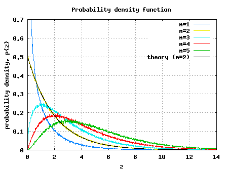
While trying to derive the theoretical bit error rate (BER) for BPSK modulation in a Rayleigh fading channel, I realized that I need to discuss chi square random variable prior. What is chi-square random variable? Let there be independent and identically distributed Gaussian random variables with mean and variance and we form a new random…
Are you bothered by speed of the speed of the simulations which you develop in Matlab/Octave? I was not bothered much, till I ran into the Viterbi decoder. If you recall, the Matlab/Octave simulation script for BER computation with hard soft decision Viterbi algorithm provided in post Viterbi with finite survivor state memory took around…
In this post, we will derive the theoretical equation for bit error rate (BER) with Binary Phase Shift Keying (BPSK) modulation scheme in Additive White Gaussian Noise (AWGN) channel. The BER results obtained using Matlab/Octave & Python simulation scripts show good agreement with the derived theoretical results. System Model Transmitter With Binary Phase Shift Keying…
Question 11 on signals from GATE (Graduate Aptitude Test in Engineering) 2012 Electronics and Communication Engineering paper. Q11. The unilateral Laplace transform of is . The unilateral Laplace transform ofis (A) (B) (C) (D) Solution From the definition of Laplace transform for a function defined for all real numbers is, , where with real numbers and . To find the Laplace…
In the recent past, we have discussed three receive diversity schemes – Selection combining, Equal Gain Combining and Maximal Ratio Combining. All the three approaches used the antenna array at the receiver to improve the demodulation performance, albeit with different levels of complexity. Time to move on to a transmit diversity scheme where the information…
In two previous posts, we have derived theoretical symbol error rate for 16-QAM and 16-PSK modulation schemes. The links are: (a) Symbol error rate for 16-PSK (b) Symbol error rate for 16-QAM Given that we are transmitting the same number of constellation points in both 16-PSK and 16-QAM, let us try to understand the better…
Question 3 on Communication from GATE (Graduate Aptitude Test in Engineering) 2012 Electronics and Communication Engineering paper. Q3. In a baseband communications link, frequencies upto 3500Hz are used for signalling. Using a raised cosine pulse with 75% excess bandwidth and for no inter-symbol interference, the maximum possible signaling rate in symbols per second is, (A)…
It might be interesting to interpret the output of the fft() function in Matlab. Consider the following simple examples. fsMHz = 20; % sampling frequency fcMHz = 1.5625; % signal frequency N = 128; % fft size % generating the time domain signal x1T = exp(j*2*pi*fcMHz*[0:N-1]/fsMHz); x1F = fft(x1T,N); % 128 pt FFT figure; plot([-N/2:N/2-1]*fsMHz/N,fftshift(abs(x1F)))…