Following the request by Siti Naimah, this post discuss the bit error probability for coherent demodulation of binary Frequency Shift Keying (BFSK) along with a small Matlab code snippet.
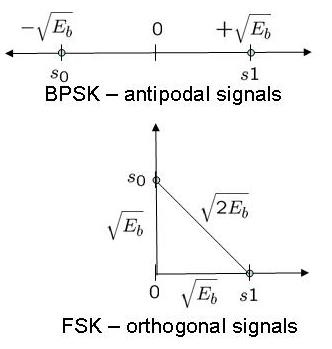
Using the definition provided in Sec 4.4.4 of [DIG-COMM-SKLAR]), in binary Frequency shift keying (BFSK), the bits 0’s and 1’s are represented by signals
and
having frequencies
and
respectively, i.e.
,
where
is the energy ,
is the symbol duration and
is an arbitrary phase (assume to be zero).
Continue reading “Bit Error Rate (BER) for frequency shift keying with coherent demodulation”