In the seminal paper Attention is All you Need (Vaswani et al 2017), the authors proposed Transformer architecture where all tokens in sequence can be processed in parallel. As the architecture process all tokens simultaneously, the concept of positional embeddings to encode the sequence information is needed. In this post, we cover few positional encoding techniques and techniques for extending the pre-trained context length.
- Sinusoidal Positional Encoding (Vaswani et al 2017)
- RoPE – Rotary Positional Encoding (Su et al., 2021)
- ALiBi – Attention with Linear Biases, Ofir Press et al 2021
- Extending pre-trained context window
- Position Interpolation (Chen et al 2023)
- NTK aware scaling (block97 2023)
- YaRN – Yet Another RoPE extensioN method (Peng et al 2023)
Sinusoidal Positional Encoding (Vaswani et al., 2017)
Prior to transformer architecture proposed in the paper Attention Is All You Need” (Vaswani et al., 2017), sequence modelling tasks such as language translation were handled using recurrent neural networks (RNNs) and recurrent variants such as LSTMs. In recurrent architectures, tokens are processed sequentially, one after another.
For a sequence of tokens
, the the hidden state evolves as,
where,
is the embedding of token at position
is the hidden state after processing token
Since tokens are processed sequentially, the order is naturally embedded into the computation. However, sequential processing prevents parallel implementation during training because a token at position cannot be processed until the previous
tokens has been consumed.
Transformer architecture
In Transformer architecture all tokens in sequence can be processed in parallel. To encode the sequence information, a positional encoding vector defined using sinusodial basis functions is defined for each element in the sequence.
In the following sections, we will go over the positional encoding scheme followed by attention scheme. In the attention layer, the interactions between the tokens (with the injected position embeddings) is used to understand the intuitions behind the definition of the positional encoding.
Positional Encoding
Each token is mapped into an embedding vector of dimension as,
Stacking all the all the embedding vectors for the sequence of length ,
The position embedding at token position
is defined as :
Positional embedding can be visualized as even & odd dimensions having sine/cosine terms and with multiple frequencies across the dimension ,
Stacking all the all the positional encoding vectors for the sequence of length ,
To encode the sequence information, postitional embeddings are added into the token embeddings.
The combined input matrix capturing the sequence of token embedding and position encoding is defined as,
Self-attention layer
The transformer architecture models interactions between all tokens using the self-attention mechanism. The combined input matrix containing token embeddings and positional encoding is projected into three learned representations called query, key and value as,
where, the learned matrices ,
and
project the token embeddings into different representation spaces.
Broadly,
(query) captures what information a token is searching for
(key) captures what information a token contains
(value) contains the information passed forward to the next layer
The interaction between every pair of tokens is computed through the query-key similarity matrix,
where the element measures how strongly token
attends to token
,
The interaction score is normalized by the key dimension and converted into attention weights using softmax (refer post Gradients for multi class classification with Softmax),
The output of the attention layer is computed as,
Each token representation is updated by aggregating information from all other tokens in the sequence.
Multi-head attention
Instead of using a single attention computation, transformer architecture employs multiple attention heads, where each head learns different relationships between tokens.
For attention head , the query, key and value projections are computed as,
Each head independently computes self-attention as,
The outputs of all heads are concatenated and projected as,
where denotes the number of attention heads.
Using multiple attention heads enables the model to simultaneously learn different relationships such as local context, long-range dependencies, syntax and semantics.
Stacking multiple transformer layers
The first layer takes the position encoded token embeddings as input,
The transformer architecture consists of multiple stacked attention layers. The output of one layer is passed as the input to the next layer, progressively refining the token representations.
If the input to layer is
, then the output of the transformer block is defined as,
where denotes the transformer block consisting of
- multi-head self-attention,
- feed-forward network,
- residual connections (refer paper Deep Residual Learning for Image Recognition, He et al 2015) and
- layer normalization (refer paper Layer Normalization, Lei Ba et al 2016)
Expanding the operations,
where,
denotes the multi-head attention operation
denotes the position-wise feed-forward network (see
denotes layer normalization
After stacked transformer layers, the final representation becomes,
Parameters in Sinusoidal Positional Encoding
In the additive sinusoidal Positional encoding described in the previous section, authors makes several key design choices, namely
- sinusoidal basis functions
- Exponentially spaced frequencies
- Emperically chosen base frequency
In the rest of the section, let us explore the intuitions and rationale behind some of the choices.
Need for sinusoidal basis function
To understand the rationale for sine and cosine terms in positional embedding, let us consider the input to the attention block for a token at ,
In the attention layer, the interaction between two tokens at position and
is computed as,
Assuming that the terms and
are identity matrices, the score can be approximated as,
Taking the position interaction term,
Applying the trignometric identity,
the position interaction term simplifies to
The position interaction term depends only on the relative distance between the tokens .
The choice of using sine and cosine terms in the position encoding, leverages the sinusoidal identity makes the position interaction term
to a decaying function which depends only on the relative distance
between tokens.
Normalized positional encoding terms
Let us define the normalized position interaction terms as
Plot of the normalized positional encoding terms
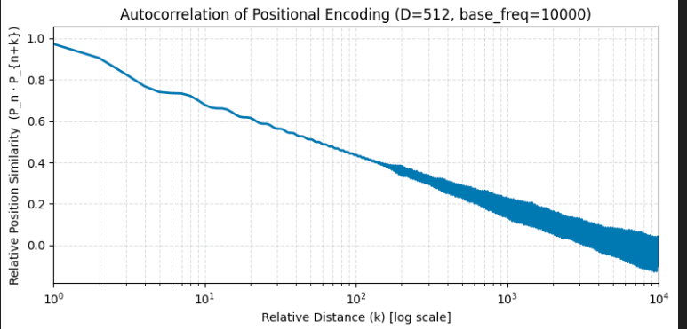
code @ positional_encoding/autocorrelation_positional_encoding.ipynb
Can see that , which captures the relative positional similarity (autocorrelation of positional encoding), exhibits an overall decaying envelope as the distance increases due to multiple frequency components being out of phase. The overall decaying trend indirectly encodes information about the relative distance between tokens.
Need for multiple frequencies
In the position encoding, multiple frequencies are chosen for various dimension as
where, the frequencies are spaced exponentially as
If only a single frequency is chosen, the relative position encoding term becomes periodic. This means different relative distance can produce identical positional similarities which causes ambiguity. Plotting the normalised positional similarity term for different number of frequency counts, can see that :
- with few frequencies (low D) : stronger oscillations
- with more frequencies (higher D) : smoother decay
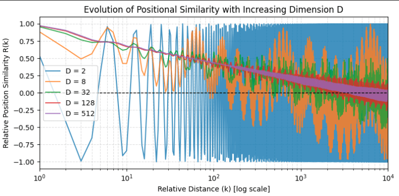
Summarising, by combining multiple frequencies, the broad intuition is :
- high frequencies capture local relative distances
- low frequencies capture the long range distances
Together, they increase the probability of each relative distance having a unique signature enabling the model to distinguish near by and far away tokens.
code @ positional_encoding/multiple_frequencies_positional_encoding.ipynb
Thus, the use of multiple exponentially spaced frequencies allows the model to encode position as a combination of signals at different scales, enabling robust representation of both local and global structure.
The choice of the constant 10,000
The choice of 10,000 as the base in the geometric progression of frequencies was an empirical engineering decision.
The positional encoding uses frequencies
which span from high-frequency components (short wavelengths) to low-frequency components (long wavelengths).
a) At (shortest wavelength):
The angular frequency is , giving a wavelength of
This short wavelength changes rapidly across nearby positions, helping the model distinguish tokens that are close to each other.
b) At (longest wavelength):
The angular frequency is approximately
giving a wavelength of
This long wavelength varies slowly across positions, helping the model encode coarse distinctions between tokens that are far apart.
Thus, the choice of 10,000 creates a spectrum of frequencies that provides both local positional resolution and long-range positional awareness.
The plot of autocorrelation of positional encoding for different base frequencies of 1000, 10000 (default) and 100000 is below.
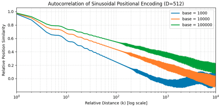
Based on the autocorrelation plot, handwaving explanation for the choice of the base frequency, and on hindsight that typical sequence lengths around the 2017 ish were around 512 tokens,
- With a base of 1000, the relative positional similarity decays more rapidly, dropping below about 0.2 at a relative distance near 100 tokens.
- With a base of 10,000, the decay is slower, and the same similarity threshold is reached only around 600 tokens.
- When the base is increased further to 100,000, the decay becomes even slower, but the lower slope reduces the separation of tokens which are close by.
So, a base of 10,000 appears to be a practical compromise between distinguishing nearby tokens and retaining information across the full training context.
Code @ positional_encoding/base_frequency_positional_encoding.ipynb
RoPE – Rotary Positional Encoding (Su et al., 2021)
In the paper RoFormer: Enhanced Transformer with Rotary Position Embedding“Su et. al 2021, the authors proposed a multiplicative approach for positional encoding instead of the additive approach for sinusoidal positional encoding.
The token embedding be of dimension , and defined as :
The token embedding at position is grouped into adjacent dimension pairs, i.e .
. The token embedding at position
is first projected into query and key representations using learned projection matrices
and
.
The query and key vectors are then grouped into adjacent dimension pairs, i.e., and
.
The rotation matrix for the pair is defined as
where,
The complete rotation matrix for positional encoding is formed by stacking these 2×2 rotation blocks across the diagonal, where each 2×2 block rotates a pair of embedding dimensions with a different angular frequency.
The rotary positional encoding is then applied to the query and key vectors as,
Expanding the matrices for ,
Similarly, the rotated query and key vectors for the token at position are defined as
Note :
Unlike sinusoidal positional encoding, which is added once to the input embeddings, RoPE is applied inside the self-attention block by rotating the query and key vectors. Since each transformer layer contains a self-attention block, the rotation operation is applied at every attention layer of the transformer architecture.
Interaction terms
In the attention layer, the interaction between two tokens at position and
is computed as
.
For intuition, assuming that the terms and
are identity matrices. Then the query and key terms simplify to
With this assumption, the score is approximated as,
Expanding the terms,
Let us find the score consider onlying the first frequency pair ,
Expanding the multiplication terms,
Grouping common terms,
Applying the trigonometric identities,
the interaction term corresponding to the frequency becomes
Since and
, the term simplifies to
Notice the key result that sine and cosine terms depend only on , and hence the interaction term depends only on the relative distance.
Extending for all frequencies, for the frequency pair , the interaction term becomes
Summing across all frequency pairs, the overall interaction score becomes
Similar to the additive positional encoding defined earlier, the interaction term in multiplicative positional encoding defined in RoPE also depends only on the relative distance between tokens .
However, unlike additive sinusoidal positional encoding, multiplicative positional encoding in RoPE does not introduce token-position cross interaction terms such as .
Complex Number Interpretation
The derivation for rotary positional encoding using explicit matrix multiplication can be expressed compactly using complex numbers. The token embedding at position is grouped into adjacent dimension pairs, i.e.
, where each pair can be represented as a complex number
where,
is the imaginary unit.
The rotary positional encoding is applied as a complex phase rotation,
Thus, the rotated embedding becomes,
Expanding the multiplication terms,
Since ,
Comparing the real and imaginary components, we observe that this is identical to the math derived earlier.
Interaction terms
In the attention layer, the interaction between two rotated token embeddings at positions and
can be written using complex number representation.
For simplicity, assuming the query and key projection matrices are identity matrices, the rotated embedding pair at frequency is expressed as
The interaction score is computed using the complex conjugate of the second term and taking the real-valued component of the output,
with,
the interaction term becomes
The absolute token position cancels out, leaving only the relative token distance
.
Normalized Positional Encoding
Let us define the embedding interaction term as,
where,
-
is the embedding similarity magnitude
is the embedding dependent phase difference
To isolate the positional component independent of the token embedding, consider
- embedding interactions are normalized i.e.
- embedding interaction phase effects are not there i.e.
With this the score simplifies to,
Then the normalized positional encoding over all the dimensions is,
This is identical to the sinusoidal positional encoding defined earlier.
ALiBi – Attention with Linear Biases, Ofir Press et al 2021
In the paper “Train Short, Test Long: Attention with Linear Biases Enables Input Length Extrapolation, Ofir Press et al 2021″, authors note that both additive sinusoidal positional encoding and multiplicative rotary positional encoding (RoPE) degrade when evaluated on sequence lengths significantly longer than those seen during training.
They also note that RoPE extrapolates better than additive sinusoidal positional encoding, with potential reasons being :
- rotary positional encoding injects positional information in every layer and not just the initial one as in additive sinusoidal positional encoding
- rotary positional encoding is done only on queries (
) and keys (
) and not to values (
)
With this intuition, authors proposed Attention with Linear Bias (ALiBi), where a static non learned bias is applied to the query key dot product prior to softmax computation.
Equations
Consider a sequence of length (). In standard self-attention, the attention score between a query at position (
) and a key at position (
) is computed as
where,
is the query at position
,
, and with causal language modelling the first i keys with
and
is the head dimension
ALiBi modifies the attention score directly by adding a position-dependent linear bias . The modified attention score becomes,
where,
-
is head specific scalar fixed before training.
- for a model with
attention heads, the set of slope is geometrically spaced and starts at
.
The ALiBi paper focused on the auto-regressive causal language models, where a query at position can only attend to the first
keys. Under this causal constraint, the bias term between a query at position
and a key at position
is calculated linearly based on their directed distance:
This creates a lower triangular bias matrix, with the diagonal elements receive a penalty of 0, and the penalty grows increasingly negative as the key moves further back into the past tokens.
This relative position information is injected at every attention operation across layers by adding a position dependent bias.
toy implementation @ positional_encoding/alibi_causal_positional_encoding.ipynb
Extending pre-trained context window
Multiple approaches for extending the pre-trained context length to a higher number has emerged in literature. In the rest of the sections, we cover three approaches – scaling the token position index, scaling by a frequency dependent factor and a scheme which combines the above approaches.
Position Interpolation (Chen et al 2023)
In the paper Extending Context Window of Large Language Models via Position Interpolation, Chen et al 2023, proposes an approach to extend the context window of RoPE based LLMs which was trained for typically ~2048 tokens to around 32768 tokens (16x).
With RoPE, the rotation factor for token at position along the
the dimension is,
where,
With Position Interpolation, the rotation factor for token position is scaled by a factor
, to become
where,
is the context length for which the model is trained
is the desired context length
NTK aware scaling (bloc97, 2023)
In the reddit post (link here) author bloc97 proposed an alternate way to extend to longer context lengths of RoPE based Large Language Models (LLMs). The key intuition comes from Neural Tangent Kernel (NTK) perspective of neural networks which suggested that neural networks are more sensitive to distortions in high frequencies than low frequency ones.
So instead of uniformly compressing all frequencies as in Positional Interpolation (PI), NTK aware scaling applies a frequency dependent scaling.
This is achieved by by introducing a frequency dependent scaling where highest frequency dimension is preserved, and progressively scaling lower frequencies, till reaching the scaling factor
for the lowest frequency
.
Equations
The base frequency in RoPE is defined as,
To scale the context window by factor , the base
is modified as,
Substituting,
For highest frequency (), the scale modifier is
, preserving the high frequency local positional context.
For the lowest frequency (), the scale factor is
, scaling the lowest frequency by the desired scaling factor
.
toy implementation @
positional_encoding/pi_ntk_aware_scaling.ipynb
YaRN – Yet Another RoPE extensioN method (Peng et al 2023)
In the paper YaRN: Efficient Context Window Extension of Large Language Models, Peng et al 2023, authors noted the following limitations :
- As the Position Interpolation scales all dimensions (frequencies) by equally by a factor
, it alters the high frequency components of RoPE
- The NTK aware scaling alleviated this to large extend by scaling high frequencies less and low frequencies more. However, identifying the optimal base frequency has to be found emperically and increasing the difficulty and cost for a fine tuned model.
To address this, authors proposed NTK by parts approach described below
NTK by parts
Let the wavelength at dimension is defined as,
Authors observe that, dimensions where the wavelength is longer than the maximum context length seen during pre-training captures the absolute positional information. However, for the dimensions where wavelength is short, it typically captures the relative positional information.
Equations
Defining the ratio between pre-trained context length and wavelength
at dimension
as,
Based on the ratio, the following constraints are defined :
- Do not interpolate for the dimensions whose wavelength
is smaller than the pre trained context length
- Do the interpolation for the dimensions whose wavelength
- For the dimensions in between, have a bit of both
Capturing this in equations,
where,
is the scale factor to increase the context length from pre-trained length
is a ramp function defined as
are thresholds to be tuned.
In the paper, authors proposed on the Llama family of models.
Pluggin in numbers,
for a pre-trained context length of and scaling to by
i.e. to extend the context length to
.
| Ratio | Wavelength | Remark |
|---|---|---|
|
|
| Interpolation |
|
|
| Linear transition |
|
| No interpolation. |
toy implementation @
positional_encoding/yarn_scaling.ipynb
Attention scaling
In addition to the frequency scaling methods described above, authors propose that scaling the attention helps lower the perplexity of the model.
The scaled attention is defined as,
where,
The equation for temperature scaling is found by fitting at the lowest perplexity against different values of
.
Summary
This post covers the following :
- the transformer positional encodings from additive sinusoidal vectors to multiplicative rotary matrices (RoPE) and static linear attention biases (ALiBi).
- Focuses on how their mathematical interactions capture relative token distance.
- Discuss the context-extension methods like Position Interpolation, NTK-Aware Scaling, and YaRN .
- Code snippets for each of the scheme is provided.