We have discussed about probable transmit pulse shaping filter and have observed that raised cosine filtering filtering allows a simpler implementation, albeit at the cost of increased bandwidth. Let us know understand the eye diagram, which is a useful graphical tool to quantify the degradation of the signal due to filtering.
Eye diagram
An eye diagram is generated in an oscilloscope operating in the persistence mode by observing the output of the filter with the symbol timing serving as the trigger. The observation window can be set as 2 times the symbol period. (Refer. Section 5.1.3 in [DIG-COMM-BARRY-LEE-MESSERSCHMITT]).
When the input data is random, the eye diagram which consists of many overlapped traces of the signal captures visually all the paths which the waveform takes.
Simulation script
Matlab/Octave script for simulating the eye diagram plot. The code performs the following
(a) Defines random BPSK modulated symbols (+1’s and -1’s)
(b) Defines two raised cosine filters with = 0.5,
= 1
(c) Upsamples the transmit sequence by zero insertion
(d) Convolves the upsampled transmit sequence with the filter
(e) Overlays the time domain samples to plot the eye diagram
Click here to download: Matlab/Octave script for ploting the eye diagram
Update
25th May 2008
Corrected the issue. Modified the code to handle division by zero.
(a) for
and
(b) for
(Thanks to the article in RFDesign.com, The care and feeding of digital, pulse-shaping filter, Ken Gentile)
19th May 2008
It has been brought to my attention that the code is unable to plot the eye diagram accurately in Matlab environment. The difference is because my version of Octave seems to handle the division by numbers close to zero cleanly, where as Matlab insists on returning Inf. I will fix the code and release an update. sorry for the inconvenience.

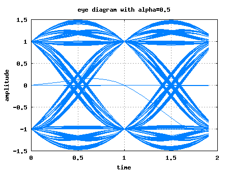
Figure: Eye diagram following raised cosine filtering with = 0.5
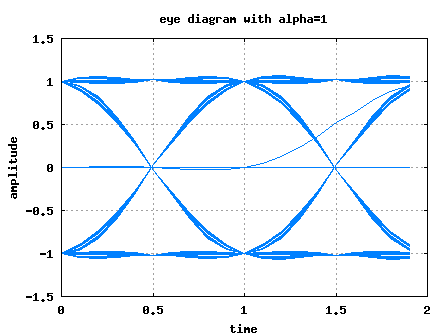
Figure: Eye diagram following raised cosine filtering with = 1
As can be observed from the above figures, the above waveform has a shape similar to the human eye and hence the name eye diagram. 🙂
Observations
1. For increasing the margin for error free transmission, the vertical opening of the eye should be more. In the presence of inter-symbol interference, the vertical opening of the eye reduces, thus increasing the probability of error.
2. The ideal sampling instant is the point where the vertical eye opening is maximum.
3. Smaller horizontal eye opening means implies more sensitivity to timing errors.
Note:
From the above figures, it can be observed that the horizontal eye opening with =0.5 is smaller than with
=1.
Reason: The tails of the raised cosine filter with =1 dies away faster than the case where
=0.5. Hence error in timing cause a bigger performance degradation for
=0.5 than for
=1 scenario. However, the flip side of using
=1 is the increased bandwidth required for transmission.
Reference
[DIG-COMM-BARRY-LEE-MESSERSCHMITT] Digital Communication: Third Edition, by John R. Barry, Edward A. Lee, David G. Messerschmitt

Hello Krishna, how do i plot the eye diagram for OFDM system? upsample->IFFT->adding timing offset->downsample->FFT->plot the eye diagram. Is it correct?
@linkin8834: Hmm… well, eye diagram is plotted on the time domain waveform getting overlayed every symbol period. For OFDM waveform with a Gaussian like distribution for the time domain, do not expect the eye diagram to carry useful information.
I am doing ofdm simulation and trying to use a eye diagram to compare the single carrier and subcarrier in multipath.
However, I don’t know how to delay the output.
For example, overall output = r(t)+0.5r(t-5us)+0.2r(t-10us) where r(t) is the signal after convolution.
@Cedric: Assuming that your samples are 5us apart, conv(rt,[1 0.5 0.2]) helps?
What is the effect of sampling time offset in the error vector magnitude? Does the sampling time offset react to changes in roll off factor?
@Theeksha: The presence of sampling time offset increases the error vector magnitude. Ideally we would like to sample at the maximum vertical eye opening, but in the presence of sampling time offset, we will drift away from the maximum eye opening window.
Hi Krishna,
I finally removed the horzontal curves in the middle of the eye diagram. Thanks
why you have line en between ?
please help me
i want code for ber for bpsk using raised cosine filter
@pravindra kumar: I have not discussed the BER with raised cosine filter case, however you can find the BER with rectangular filter at https://dsplog.com/2009/05/08/ber-with-matched-filtering/
Hi Krishna,
I have a question regarding the plot of eye diagram that you’ve shown.
You said its plotted for two symbols and the eye opening seems to be at
the center of the diagram(at completion of first unit interval). So is plotted
like half of previous bit,current bit and half of future ?
Hi Mr krishna ,
I don’t understand the utility of “upsampling the transmit sequence ”
what will happen if we did not add the zeros to the sequence ?
I wonder if there is some links clarifying this idea .
thank you very much.
@Fahmi: With a sampling frequency of fs, we can ‘see’ frequencies from [-fs/2 to fs/2). Typically, we would want to control a bigger bandwidth compared to the original transmit sequence. Hence we do upsampling.
krishna can u help me…why the graph of BER vs SNR in BPSK in theoretical and simulation is same..Whats the reason about it..
@nyna: We want to have our simulations to be in good agreement with theory, no? It helps us confirm that we were able to model all the equations correctly. 🙂
@Prashant: All the data which we need to obtain can be observed by plotting for two symbol periods – width of the eye opening, transition edges etc. Ofcourse, nothing stops us from plotting for 3 (or more) symbol periods….
Glad that you are finding this site useful. Typically books do not cover these small details. To return the favour, you can refer this site to your friends/colleagues. Thanks.
You have plotted it for two symbol period. Is that a rule or it varies i mean eye-diagram by definition assumes two symbol period? Actually I could not find any material which deals with implementation of eye-diagram except yours and in the books they don’t mention these details.
@Prashant: You are right. x-axis is the time. I have assumed sampling frequency of fs=10 and plotted for two symbol periods.
Hi,
Thanks for the nice article. I tried your matlab code, but I have some confusion. Can you elaborate your x axis in the code i.e. time axis? I mean, what is symbol rate and bit rate, why have you plotted this for 20 time instants, (i guess 20 = 2*fs in the code)?
TIA
very good!