June 2007 - DSP LOG

Interpreting the output of fft() operation in Matlab

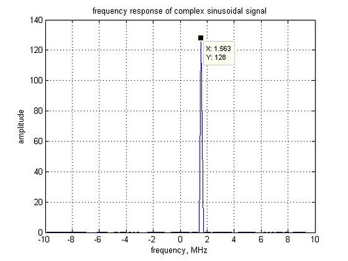
It might be interesting to interpret the output of the fft() function in Matlab. Consider the following simple examples.

fsMHz = 20; % sampling frequency
fcMHz = 1.5625; % signal frequency
N = 128; % fft size
% generating the time domain signal
x1T = exp(j*2*pi*fcMHz*[0:N-1]/fsMHz);
x1F = fft(x1T,N); % 128 pt FFT
figure;
plot([-N/2:N/2-1]*fsMHz/N,fftshift(abs(x1F))) ; % sub-carriers from [-128:127]
xlabel('frequency, MHz')
ylabel('amplitude')
title('frequency response of complex sinusoidal signal');

Continue reading “Interpreting the output of fft() operation in Matlab”

First order digital PLL for tracking constant phase offset

Considering a typical scenario where there might exist a small phase offset between local oscillator between the transmitter and receiver.

Figure 1 : Transmitter receiver with constant phase offset

In such cases, it might be desirable to estimate and track the phase offset such that the performance of the receiver does not degrade.

Continue reading “First order digital PLL for tracking constant phase offset”