For curve fitting using linear regression, there exists a minor variant of Batch Gradient Descent algorithm, called Stochastic Gradient Descent.
In the Batch Gradient Descent, the parameter vector  is updated as,
 - y^j\]x_i^j\end{array}) .
.
(loop over all elements of training set in one iteration)
For Stochastic Gradient Descent, the vector gets updated as, at each iteration the algorithm goes over only one among  training set, i.e.
 - y^j\]x_i^j\end{array}) .
.
When the training set is large, Stochastic Gradient Descent can be useful (as we need not go over the full data to get the first set of the parameter vector )
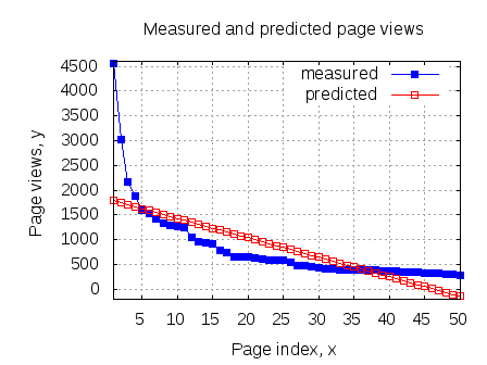
For the same Matlab example used in the previous post, we can see that both batch and stochastic gradient descent converged to reasonably close values.
Matlab/Octave code snippet
clear ;
close all;
x = [1:50].';
y = [4554 3014 2171 1891 1593 1532 1416 1326 1297 1266 ...
	1248 1052 951 936 918 797 743 665 662 652 ...
	629 609 596 590 582 547 486 471 462 435 ...
	424 403 400 386 386 384 384 383 370 365 ...
	360 358 354 347 320 319 318 311 307 290 ].';
%
m = length(y); % store the number of training examples
x = [ ones(m,1) x]; % Add a column of ones to x
n = size(x,2); % number of features
theta_batch_vec = [0 0]';
theta_stoch_vec = [0 0]';
alpha = 0.002;
err = [0 0]';
theta_batch_vec_v = zeros(10000,2);
theta_stoch_vec_v = zeros(50*10000,2);
for kk = 1:10000
	% batch gradient descent - loop over all training set
	h_theta_batch = (x*theta_batch_vec);
	h_theta_batch_v = h_theta_batch*ones(1,n);
	y_v = y*ones(1,n);
	theta_batch_vec = theta_batch_vec - alpha*1/m*sum((h_theta_batch_v - y_v).*x).';
	theta_batch_vec_v(kk,:) = theta_batch_vec;
	%j_theta_batch(kk) = 1/(2*m)*sum((h_theta_batch - y).^2);

	% stochastic gradient descent - loop over one training set at a time
	for (jj = 1:50)
		h_theta_stoch = (x(jj,:)*theta_stoch_vec);
		h_theta_stoch_v = h_theta_stoch*ones(1,n);
		y_v = y(jj,:)*ones(1,n);
		theta_stoch_vec = theta_stoch_vec - alpha*1/m*((h_theta_stoch_v - y_v).*x(jj,:)).';
		%j_theta_stoch(kk,jj) = 1/(2*m)*sum((h_theta_stoch - y).^2);
		theta_stoch_vec_v(50*(kk-1)+jj,:) = theta_stoch_vec;
	end
end

figure;
plot(x(:,2),y,'bs-');
hold on
plot(x(:,2),x*theta_batch_vec,'md-');
plot(x(:,2),x*theta_stoch_vec,'rp-');
legend('measured', 'predicted-batch','predicted-stochastic');
grid on;
xlabel('Page index, x');
ylabel('Page views, y');
title('Measured and predicted page views');

j_theta = zeros(250, 250);   % initialize j_theta
theta0_vals = linspace(-2500, 2500, 250);
theta1_vals = linspace(-50, 50, 250);
for i = 1:length(theta0_vals)
	  for j = 1:length(theta1_vals)
		theta_val_vec = [theta0_vals(i) theta1_vals(j)]';
		h_theta = (x*theta_val_vec);
		j_theta(i,j) = 1/(2*m)*sum((h_theta - y).^2);
    end
end
figure;
contour(theta0_vals,theta1_vals,10*log10(j_theta.'))
xlabel('theta_0'); ylabel('theta_1')
title('Cost function J(theta)');
hold on;
plot(theta_stoch_vec_v(:,1),theta_stoch_vec_v(:,2),'rs.');
plot(theta_batch_vec_v(:,1),theta_batch_vec_v(:,2),'kx.');
The converged values are :
 .
.

From the below plot, we can see that Batch Gradient Descent (black line) goes straight down to the minima, whereas Stochastic Gradient Descent (red line) keeps hovering around (thick red line) before going down to the minima.

References
An Application of Supervised Learning – Autonomous Deriving (Video Lecture, Class2)
CS 229 Machine Learning Course Materials