My understanding of the CORDIC (Co-ordinate Rotation by DIgital Computer) thanks to the nice article in [DSPGURU-CORDIC].
Category: DSP
Defines typical signal processing blocks like – CORDIC’s, polyphase filters etc
Straight line fit using least squares estimate
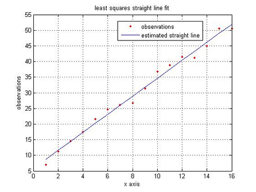
Two points suffice for drawing a straight line. However we may be presented with a set of data points (more than two?) presumably forming a straight line. How can one use the available set of data points to draw a straight line?
A probable approach is to draw a straight line which hopefully minimizes the error between the observed data points and estimated straight line.
where
is the observed data points and
is the points from estimated straight line.
Continue reading “Straight line fit using least squares estimate”
Interpreting the output of fft() operation in Matlab
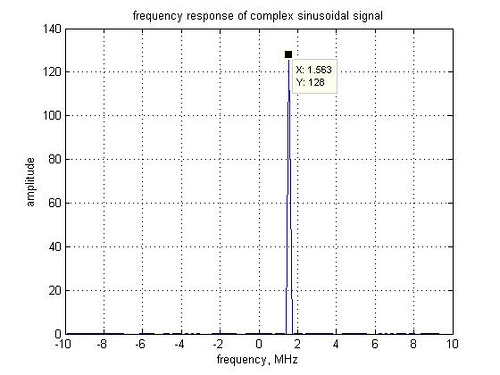
It might be interesting to interpret the output of the fft() function in Matlab. Consider the following simple examples.
fsMHz = 20; % sampling frequency
fcMHz = 1.5625; % signal frequency
N = 128; % fft size
% generating the time domain signal
x1T = exp(j*2*pi*fcMHz*[0:N-1]/fsMHz);
x1F = fft(x1T,N); % 128 pt FFT
figure;
plot([-N/2:N/2-1]*fsMHz/N,fftshift(abs(x1F))) ; % sub-carriers from [-128:127]
xlabel('frequency, MHz')
ylabel('amplitude')
title('frequency response of complex sinusoidal signal');
Continue reading “Interpreting the output of fft() operation in Matlab”
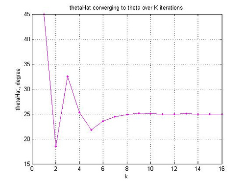
First order digital PLL for tracking constant phase offset
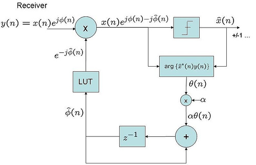
Considering a typical scenario where there might exist a small phase offset between local oscillator between the transmitter and receiver.
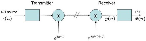
Figure 1 : Transmitter receiver with constant phase offset
In such cases, it might be desirable to estimate and track the phase offset such that the performance of the receiver does not degrade.
Continue reading “First order digital PLL for tracking constant phase offset”
Using Toeplitz matrices in MATLAB
The definition of Toeplitz matrix from [1] is:
A matrix is said to be Toeplitz if the elements
are determined completely by the difference
.