Batch Gradient Descent

I happened to stumble on Prof. Andrew Ng’s Machine Learning classes which are available online as part of Stanford Center for Professional Development. The first lecture in the series discuss the topic of fitting parameters for a given data set using linear regression.  For understanding this concept, I chose to take data from the top 50 articles of this blog based on the pageviews in the month of September 2011.

Notations

Let

be the number of training set (in our case top 50 articles),

be the input sequence (the page index),

be the output sequence (the page views for each page index)

be the number of features/parameters (=2 for our example).

The value of corresponds to the training set

Let us try to predict the number of page views for a given page index using a hypothesis, where is defined as :

where,

is the page index,

.

Linear regression using gradient descent

Given the above hypothesis, let us try to figure out the parameter which minimizes the square of the error between the predicted value and the actual output for all values in the training set i.e.

Let us define the cost function as,

.

The scaling by fraction is just for notational convenience.

Let us start with some parameter vector , and keep changing the to reduce the cost function , i.e.

.

The parameter vector after algorithm convergence can be used for prediction.

Note :

1. For each update of the parameter vector , the algorithm process the full training set. This algorithm is called Batch Gradient Descent.

2. For the given example with 50 training sets, the going over the full training set is computationally feasible. However when the training set is very large, we need to use a slight variant of this scheme, called Stochastic Gradient Descent. We will discuss that in another post.

3. The proof of the derivation of  involving differential with will be of interest. We will discuss that in another post.

Matlab/Octave code snippet

clear ;
close all;
x = [1:50].';
y = [4554 3014 2171 1891 1593 1532 1416 1326 1297 1266 ...
	1248 1052 951 936 918 797 743 665 662 652 ...
	629 609 596 590 582 547 486 471 462 435 ...
	424 403 400 386 386 384 384 383 370 365 ...
	360 358 354 347 320 319 318 311 307 290 ].';

m = length(y); % store the number of training examples
x = [ ones(m,1) x]; % Add a column of ones to x
n = size(x,2); % number of features
theta_vec = [0 0]';
alpha = 0.002;
err = [0 0]';
for kk = 1:10000
	h_theta = (x*theta_vec);
	h_theta_v = h_theta*ones(1,n);
	y_v = y*ones(1,n);
	theta_vec = theta_vec - alpha*1/m*sum((h_theta_v - y_v).*x).';
	err(:,kk) = 1/m*sum((h_theta_v - y_v).*x).';
end

figure;
plot(x(:,2),y,'bs-');
hold on
plot(x(:,2),x*theta_vec,'rp-');
legend('measured', 'predicted');
grid on;
xlabel('Page index, x');
ylabel('Page views, y');
title('Measured and predicted page views');

The computed values are

.

With this hypotheses, the predicted page views is shown in the red curve (in the below plot).

In matlab code snippet, kept the number of step of gradient descent blindly as 10000. One can probably stop the gradient descent when the cost function is small and/or when rate of change of is small.

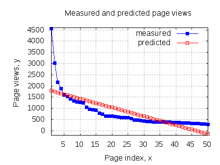
Couple of things to note :

1. Given that the measured values are showing an exponential trend, trying to fit a straight line does not seem like a good idea. Anyhow, given this is the first post in this series, I let it pass. 🙂

2. The value of controls the rate of convergence of the algorithm. If is very small, the algorithm takes small steps and takes longer time to converge. Higher value of causes the algorithm to take large steps, and may cause algorithm to diverge.

3. Have not figured how to select value suitable (fast convergence) for the data set under consideration. Will figure that out later.

Plotting the variation of for different values of

clear;
j_theta = zeros(250, 250);   % initialize j_theta
theta0_vals = linspace(-5000, 5000, 250);
theta1_vals = linspace(-200, 200, 250);
for i = 1:length(theta0_vals)
	  for j = 1:length(theta1_vals)
		theta_val_vec = [theta0_vals(i) theta1_vals(j)]';
		h_theta = (x*theta_val_vec);
		j_theta(i,j) = 1/(2*m)*sum((h_theta - y).^2);
    end
end
figure;
surf(theta0_vals, theta1_vals,10*log10(j_theta.'));
xlabel('theta_0'); ylabel('theta_1');zlabel('10*log10(Jtheta)');
title('Cost function J(theta)');
figure;
contour(theta0_vals,theta1_vals,10*log10(j_theta.'))
xlabel('theta_0'); ylabel('theta_1')
title('Cost function J(theta)');

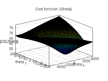
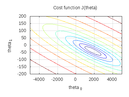
Given that the surface() plot is bit unwieldy in my relatively slow desktop, using contour() plot seems to be a much better choice. Can see that the minima of this cost function lies near the computed values of

.

References

An Application of Supervised Learning – Autonomous Deriving