In typical wireless system simulations, there is a need to model the phase noise profile of the local oscillator. For eg, the phase noise profile of the oscillator can be of the shape described in the post on Phase Noise Power Spectral Density to Jitter. While looking around for example Matlab code, found two references [1, 2] which uses the approach of defining the phase noise profile in frequency domain, and then using ifft() to convert to the time domain samples. This post gives a brief overview of the modeling and provides an example Matlab/Octave code.
Modeling
a) Assume a system with sampling frequency Hz and having
samples. In frequency domain we can define
in steps of
Hz.
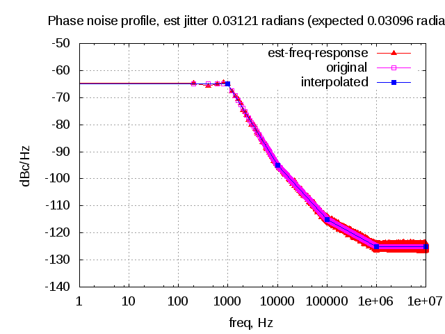
b) Consider a phase noise profile defined as follows :
| freq | PSD, dBc/Hz |
| 0 | -65 |
| 1kHz | -65 |
| 10kHz | -95 |
| 100kHz | -115 |
| 1MHz | -125 |
| 10MHz | -125 |
Table : Example phase noise profile
From the phase noise profile, using linear interpolation (in log10 of the frequency axis), to find the phase noise power spectral density for frequencies from in steps of
Hz.
c) Generate a white Gaussian noise sample of length and scale it with the phase noise power spectral density
(Scaling by is to normalize the resolution bandwidth to unity)
d) Use ifft() to find the time domain samples.
e) On the rel samples obtained from step (d), take to form the time domain phase noise samples.
Note :
When x is small, .
Example Matlab script
% Script for simulating the an example phase noise profile
% ----------------------------------------------------------

clear all; close all;
fs_Hz    = 20e6;
N        = 10^5;
nIter    = 100;

% phase noise profile
psd_f_hz           = [  0  1e3  1e4  1e5  1e6  10e6];
psd_val_dbc_per_hz = [-65  -65  -95 -115 -125  -125];

% defining the frequency vector
freq_v_Hz = [0:N/2]/N*fs_Hz;
delta_f   = fs_Hz/N;
slope    = [psd_val_dbc_per_hz(2:end) - psd_val_dbc_per_hz(1:end-1) ]./...
		(log10(psd_f_hz(2:end)) - log10(psd_f_hz(1:end-1)));
constant = 10.^(psd_val_dbc_per_hz(1:end-1)/10).* ...
		(psd_f_hz(1:end-1).^(-slope/10));
integral = constant.*(psd_f_hz(2:end).^(1+slope/10) - ...
			psd_f_hz(1:end-1).^(1+slope/10) )./(1+slope/10);
%% finding the rms jitter
% finding index with slope == -10
idx = find(slope==-10);
integral(idx) = constant(idx).*(log(psd_f_hz(idx+1)) - log(psd_f_hz(idx)));
rms_jitter_radians  = sqrt(2*integral);
integrated_jitter_radians = sqrt(2*sum(integral))

% interpolating the phase noise psd values
psd_ssb_dB = -Inf*ones(1,N/2+1); % from [0:N/2]
for ii=1:length(psd_f_hz)-1
   [tt1 fl_idx ] = (min(abs(psd_f_hz(ii) - freq_v_Hz)));
   [tt2 fr_idx ] = (min(abs(psd_f_hz(ii+1) - freq_v_Hz)));
   fvec = [freq_v_Hz(fl_idx):delta_f:freq_v_Hz(fr_idx)];
   pvec = slope(ii)*log10(fvec+eps) + psd_val_dbc_per_hz(ii) - slope(ii)*log10(psd_f_hz(ii)+eps);
   psd_ssb_dB(fl_idx:fr_idx) = pvec;
end

% forming the full vector from [-N/2:-1 0:N/2-1 ]/N*fs_Hz
psd_dB                  = -Inf*ones(1,N);
psd_dB([-N/2:-1]+N/2+1) = psd_ssb_dB([N/2+1:-1:2]);
psd_dB([0:N/2-1]+N/2+1) = psd_ssb_dB(1:N/2);

psd_linear = 10.^(psd_dB/20);

for (jj = 1:nIter)
   % defining frequency vector
   phase_noise_freq       = 1/sqrt(2)*(randn(1,N) + j*randn(1,N));
   phase_noise_freq_scale = N*sqrt(delta_f)*phase_noise_freq;
   phase_noise_freq_psd   = phase_noise_freq_scale .*psd_linear;

   % converting to time domain
   phase_noise_td      = ifft(fftshift(phase_noise_freq_psd));
   pn_td               = exp(j*(sqrt(2)*real(phase_noise_td)));

   % for estimating jitter and plotting
   pn_without_carrier  = (pn_td - 1);
   est_jitter_pwr_radians(jj) = mean(pn_without_carrier.*conj(pn_without_carrier));

   hF           = 1/(N*sqrt(delta_f))*fft(pn_without_carrier,N);
   hFPwr(jj,:)  = hF.*conj(hF);
end

est_integrated_jitter_radians = sqrt(mean(est_jitter_pwr_radians));
title_str = sprintf('Phase noise profile, est jitter %2.5f radians (expected %2.5f radians)', est_integrated_jitter_radians, integrated_jitter_radians);

figure
semilogx( [-N/2:N/2-1]/N*fs_Hz, 10*log10(fftshift(mean(hFPwr))), 'r^-' );
hold on;grid on;
semilogx([0:N/2]/N*fs_Hz,psd_ssb_dB,'mp-');
semilogx(psd_f_hz,psd_val_dbc_per_hz,'bs-');
legend('est-freq-response','original','interpolated');
xlabel('freq, Hz'); ylabel('dBc/Hz');
axis([1 10e6 -140 -50]); title(title_str);
Figure : Example phase noise profile (expected and simulated)
Summary
The above approach seems to allow a way to model an arbitrary phase noise power spectral density. However, the fact that this approach needs a large ifft() of length can potentially slow down the simulation.
References
[1] Phase Noise by Alex Bar-Guy, 27 Oct 2005 (Updated 08 Dec 2005) http://www.mathworks.com/matlabcentral/fileexchange/8844-phase-noise
[2] Baseband-equivalent phase noise model, Submitted by Markus Nentwig on Dec 18 2011

great work Krishna, thank you for sharing!