Loss functions for handling class imbalance

Most of real world datasets have class imbalance, where a “majority” class dwarfs the “minority” samples. Typical examples are – identifying rare pathologies in medical diagnosis or flagging anomalous transactions to detect fraud or detecting sparse foreground objects from vast background objects in computer vision to name a few.

The machine learning models we have discussed – binary classification ^{(refer post Gradients for Binary Classification with Sigmoid)} or multiclass classification ^{(refer post Gradients for multi class classification with Softmax)} needs tweaks to learn from these imbalanced datasets. Without these adjustments, the models can “cheat” by favouring the majority class and can report a pseudo high accuracy though the class specific accuracy is low.

Different strategies have emerged over the years, and in this article we are covering the approaches listed below.

Weighted cross entropy
- Foundational baseline, where a class-specific weight factor to the standard cross-entropy loss to weight the loss based on frequency of the class.
Focal Loss for Dense Object Detection, Lin et al. (2017)
- Propose a modulating factor $(1-p_t) ^\gamma$ to the cross-entropy loss to down-weight easy/frequent examples which indirectly forces the model to focus on hard/rare examples
Asymmetric Loss for Multi-Label Classification, Ridnik et al. (2021)
- Extended the intuition of Focal Loss by having independent $\gamma$ hyper-parameter for positive and negative samples. This allows for more aggressive “pushing” of easy/frequent examples while preserving the gradient signal for hard/rare samples.
- Additionally, authors introduces a probability margin that explicitly zeros out the loss from easy/frequent samples.
Class-Balanced Loss Based on Effective Number of Samples, Cui et al. (CVPR 2019)
- Based on the intuition that there are similarities among the samples, authors propose a framework to capture the diminishing benefit when more datasamples are added to a class.
Long-tail Learning via Logit Adjustment, Menon et al. (ICLR 2021)
- Based on the foundations from Bayes Rule, authors propose that adding a class dependent offset based on the prior probabilities help the model learn to minimise the balanced error rate (the average of error rates for each class) instead of minimising global error rate.

Table of Contents

Weighted Cross Entropy

Standard Cross Entropy treats all classes equally, which becomes problematic when your dataset contains 1,000s of easy background examples but only 100s of rare foreground objects. In such cases, the majority class dominates the loss and biases the model. Weighted Cross Entropy (WCE) addresses this by assigning a static weight to each class, manually boosting the importance of rare samples.

Binary weighted Cross Entropy

For binary classification, a weighting factor $\alpha \in [0, 1]$ to the standard BCE formula is used the scale the loss.

$Weighted Binary Cross Entropy Formula$

where $\alpha$ is typically set to the inverse of the class frequency.

By setting a high $\alpha$ for the rare class (e.g., 0.9 for the 100 foreground samples) and a low weight for the frequent class (0.1 for the 1,000 background samples), ensures that the rare foreground objects provide a sufficient gradient signal during training.

Multiclass Weighted Cross Entropy

In the multiclass case with $K$ classes, the loss for a single example where $c$ is the ground-truth label is defined as:

$Multiclass Weighted Cross Entropy Formula$

Where $\alpha_c$ is a fixed weight assigned to class $c$ , typically calculated using the Inverse Class Frequency:

$Inverse Class Frequency formula$

Weighted versions of cross entropy loss is natively supported in PyTorch library as :

torch.nn.BCEWithLogitsLoss ^(refer) : using the argument pos_weight for the binary classification
torch.nn.CrossEntropyLoss ^(refer) : using the argument weight for multiclass classification.

Toy example computing the loss using the manually vs PyTorch implementation @ loss_functions_for_class_imbalance/weighted_cross_entropy.ipynb

Focal Loss (Lin et al 2017)

In the paper Focal Loss for Dense Object Detection Lin et al. (2017) , authors propose an extension to standard Cross Entropy loss to focus training on hard/rare examples. The key intuition is that by adding a probability-dependent modulating factor to the loss, the contribution of easy/frequent examples (where the estimated probability is close to the truth) is down-weighted. This indirectly forces the training to focus specifically on the hard/rare examples.

Focal loss is defined as :

$FL(y,p) = -[(1-p)^\gamma y \log(p) + p^\gamma (1-y)\log(1-p) ]$

where,

$y\in\{0,1\}$ represent the ground truth labels and
$p\in\[0,1]$ is the estimated probabilities
$\gamma$ is a hyperparameter to control the modulating factor

Note : The standard cross entropy loss for binary classification is

$CE(y,p) = -[y\log(p) + (1-y)\log(1-p) ]$

Gradients in standard Cross Entropy Loss

To understand how Focal Loss works, the gradient i.e. the derivative with respect to the model’s output logits, $z$ is explored. The model outputs a real number ${z}$ number, which is converted to a probability $p\in\[0,1]$ using the sigmoid function $\sigma(z)$ .

Using the chain rule from calculus ^{(refer wiki entry on Chain Rule)}, then the gradient of loss with respect ${z}$ $\frac{\partial {L}}{\partial z}$ is found as – gradient of loss with respect to probabilty $\frac{\partial {L}}{\partial p}$ multiplied with gradient of probability with respect to parameter $\frac{\partial p}{\partial z}$ i.e.

$\frac{\partial {L}}{\partial \mathbf{z}} = \frac{\partial {L}}{\partial p} \cdot \frac{\partial p}{\partial z}$

For standard Cross Entropy loss, as derived in the post on Gradients for Binary Classification with Sigmoid, gradient is,

$\begin{array}{lll} \frac{\partial {CE}}{\partial {p}} & = & -\left[\frac{y}{p} - \frac{1-y}{1-p} \right] \\ \frac{\partial {p}}{\partial {z}} & = & p(1-p) \\ \\ \text{then, } \\ \frac{\partial {CE}}{\partial {z}} & = & \frac{\partial {CE}}{\partial {p}} \cdot \frac{\partial {p}}{\partial {z}} \\ &=& -\left[\frac{y}{p} - \frac{1-y}{1-p} \right] \cdot p(1-p) \\ &=&-\left[y(1-p) - (1-y)p \right] \\ &=&p-y \end{array}$

The gradient is linear and depends only on the error – this means an “easy/frequent” example (where the error is small, e.g., 0.1) when summed over large number of of easy examples still contributes to the loss and can overwhelm the training.

Gradients in Focal Loss

For computing the gradients with focal loss, let us define the ground truth labels $y\in\{0,1\}$ and the model’s estimated probability $p\in\[0,1]$ as :

$Definition of pt$

where,

$y=0$ background class with 1000’s of easy/frequent examples
$y=1$ foreground class with 100’s of hard/rare examples

Taking the case of $y=1$ ,

$\begin{array}{lll} \frac{\partial {FL}}{\partial p_t} & = & -(1-p_t)^\gamma \cdot \frac{\partial }{\partial p_t}\log(p_t) - \log(p_t) \frac{\partial }{\partial p_t}(1-p_t)^\gamma \\ & = & -(1-p_t)^\gamma \cdot \frac{1}{(p_t)} + \gamma (1-p_t)^{\gamma-1}\log(p_t) \\ \end{array}$

Multiplying with $\frac{\partial {p_t}}{\partial {z}} = p_t(1-p_t)$ ,

$\begin{array}{lll} \frac{\partial {FL}}{\partial {z}} & = & \frac{\partial {FL}}{\partial {p_t}} \cdot \frac{\partial {p_t}}{\partial {z}} \\ & = & \[-(1-p_t)^\gamma \cdot \frac{1}{(p_t)} + \gamma (1-p_t)^{\gamma-1}\log(p_t) \] \cdot p_t(1-p_t) \\ & = & \[-(1-p_t)^{\gamma+1} + \gamma p_t(1-p_t)^{\gamma}\log(p_t) \] \\ & = & (1-p_t)^{\gamma}\[-(1-p_t) + \gamma p_t\log(p_t) \] \\ & = & \underbrace{(1-p_t)^{\gamma}}_{\text{scaling term}}\[\underbrace{(p_t-1)}_{\text{CE term}} + \underbrace{\gamma p_t\log(p_t)}_{\text{focal term}} \] \end{array}$

Sweeping the value of $p$ from 0 to 1 for $\gamma=2$ , the behaviour of the individual terms are as shown in the plot below.

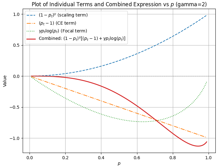
code @ focal_loss_terms.py

The model learns easy/frequent examples much faster and $p$ is close to the ground truth $y$ , which means $p_t\rightarrow 1$ . As $p_t$ approaches 1, the scaling term $(1-p_t) ^\gamma$ effectively silences the gradient.

Plugging in numbers, when the model is estimating $p_t \approx 0.99$ for the frequent examples, the throttle becomes $(1-0.99)^2 \approx 0.0001$ and the gradient from these examples is effectively silenced.

$\begin{array}{lll} \frac{\partial FL}{\partial z} & \approx &(1-p_t)^\gamma (p - y) \end{array}$

Thus the term $(1-p_t) ^\gamma$ acts as a throttle for easy/frequent examples.

The Weighting Factor $\alpha$

With the focusing parameter $\gamma$ down-weighting easy/frequent examples, the choosing class weights $\alpha$ parameter using inverse of class frequency is not preferred. To understand the intuitions, let us define $\alpha_t$ as below :

$Definition of alpha_t$

The Focal Loss including $\alpha_t$ is :

$Alpha Balanced Focal Loss$

When we go with inverse of class frequency, typically values of $\alpha$ is :

high $\alpha$ (around 0.9) for $y=1$ (hard/rare foreground class) and
low $\alpha$ (around 0.1) for $y=0$ (easy/frequent background class)

With the Focal Loss, the focusing term $(1-p_t)^\gamma$ aggressively down-weights the easy examples and the accumulated loss from the background class drops drastically. Then with high $\alpha$ the hard/rare foreground class with only 100s of examples will now dominate the gradient and can cause instability.

Therefore, as $\gamma$ is increased, $\alpha$ should be decreased. In the paper, for $\gamma=2$ , the authors found the best balance was actually $\alpha=0.25$ for the foreground class $y=1$ .

Extension to Multiclass Focal Loss

While the binary case uses a single probability $p$ , the multiclass classification involve $C$ distinct classes. In the multiclass setting, the model outputs a vector of logits, which are transformed into probabilities using the Softmax function. The estimated probability for $l^{th}$ class is :

$P_{l} = \frac{e^{z_{l}}}{\sum_{j=1}^{C} e^{z_{j}}}$

The Multiclass Focal Loss for a single example for $l^{th}$ ground truth class is,

$FL_{\text{multi class}} = -\alpha_{l} (1 - P_{l})^\gamma \log(P_{l})$

Typically $\gamma=2$ is chosen as a scalar, and the weights factor $\alpha_{l}$ is defined as a class dependent vector.

Choosing $\alpha_{l}=0.25$ for the rare classes and $\alpha_{l}=0.75$ for the frequent classes seems to be choice which can be arrived at using hyper parameter tuning. Though it is counter intuitive to give higher $\alpha$ for frequent classes, it helps to prevent their contribution from being completely throttled by the $(1-p_t)^\gamma$ term.

Toy example showing implementation of Focal Loss for binary and multi-class classification @ loss_functions_for_class_imbalance/focal_loss_binary_multiclass.ipynb

Assymetric Loss (2021)

In the focal loss definition, the same $\gamma$ is used for both background class with high count of easy examples and rare foreground class. If a higher $\gamma$ is used to throttle the gradients of easy background classes, then this also affects when the model is learning the hard foreground classes.

In the paper, Asymmetric Loss for Multi-Label Classification, Ridnik et al. (2021). authors proposed to decouple the $\gamma$ for foreground and background classes.

$L = \begin{cases} -(1-p)^{(\gamma_+)} \log(p) & \text{if } y=1 \quad \text{(hard/rare foreground class)}\\ -p^{(\gamma_-)} \log(1-p) & \text{if } y=0 \quad \text{(easy/frequent background class)} \end{cases}$

To give emphasis to the contribution of positive samples, $\gamma_- \gt \gamma_+$ .

The typical values can be $\gamma_+ =0$ so that the hard/low count positive samples behave similar to standard cross entropy loss and $\gamma_- =2$ to throttle gradients for easy/high count background classes.

Authors further propose adding a margin on the probability of easy backround classes by probability shifting which discards them when the probability is below a threshold.

$p_m= \max(p-m,0)$

with $m$ as a hyperparameter and a typical value being $m=0.2$ .

Combining both, the Assymetric Loss is defined as,

$ASL = \begin{cases} -(1-p)^{(\gamma_+)} \log(p) & \text{if } y=1 \quad \text{(hard/rare foreground class)}\\ -p_m^{(\gamma_-)} \log(1-p_m) & \text{if } y=0 \quad \text{(easy/frequent background class)} \end{cases}$

Toy implementation of assymetric loss @ loss_functions_for_class_imbalance/assymetric_loss.ipynb

Class-Balanced Loss (Yin Cui et al 2019)

In the paper Class-Balanced Loss Based on Effective Number of Samples, Cui et al. , authors argue that there will be similarities among the samples and as the number of samples increase, the probability that this sample is covered in the existing samples increases. Based on this intuition, authors propose a framework to capture the diminishing benefit when more datasamples are added to a class.

Derivation

Let us denote the effective number of samples as $E_n$ , and the total volume of this space as $N$ . Consider the case where we have $n-1$ examples and is going to sample the $n^{th}$ example. The probability that the newly sampled example to be overlapped with the previous samples is,

$p=\frac{E_{n-1}}{N}$

Expected volume with the $n^{th}$ example is,

$\begin{array}{lll}E_n & = & pE_{n-1} + (1-p)(E_{n-1}+1) \\ & = & pE_{n-1} + E_{n-1}+1 -pE_{n-1} - p \\ & = & E_{n-1} + 1-p\\ \quad \text{substituting for } p, \\ & = & E_{n-1} + 1- \frac{E_{n-1}}{N} \\ & = & \frac{NE_{n-1} + N - E_{n-1}}{N} \\ & = & 1 + \frac{N-1}{N}E_{n-1} \\ & = & 1 + \beta E_{n-1}, \quad \text{where, } \beta = \frac {N-1}{N} \end{array}$

To solve for $E_n$ , re-writing as a geometric series,

$\begin{array}{llll} n=1, & E_1 & =& 1\\ n=2, & E_2 &= & 1+\beta E_1 = 1+\beta \\ n=3, & E_3 &= & 1+\beta E_2 = 1+\beta(1+\beta) = 1+ \beta + \beta^2 \\ n=4, & E_4 &= & 1+\beta E_3 = 1+\beta(1+\beta+\beta^2) = 1+ \beta + \beta^2 + \beta^3 \\ \vdots \end{array}$

For the general $E_n$ can be written as

$\begin{array}{llllll} E_n & = & \sum_{j=1}^{n} \beta^{j-1} & = & 1 + \beta + \beta^2 + \cdots + \beta^{n-1} \end{array}$

Solving for $E_n$ ,

$\begin{array}{llllll} E_n - \beta E_n & = & (1 + \beta + \beta^2 + \cdots + \beta^{n-1}) - \beta(1 + \beta + \beta^2 + \cdots + \beta^{n-1}) \\ & = & 1-\beta^n \\ \text{solving, }\\ (1-\beta)E_n & = & 1-\beta^n \\ E_n & = & (1-\beta^n)/(1-\beta) \end{array}$

Note :

When $\beta=0$ , the effective number of samples $E_n=1$ indicating that there is no benefit in adding more samples.
When $\beta\rightarrow 1$ , the expected number of samples $E_n=n$ , indicating that each sample is treated unique.

$\begin{array}{lll} \lim_{\beta \to 1}E_n & = & \lim_{\beta \to 1}\frac{(1-\beta^n)}{(1-\beta)} \\ \text{using L' Hospitals rule, } \\ & = & \frac{-n\beta^{n-1}}{-1} & = & n \end{array}$

In the paper authors explore $\beta$ as a hyper-parameter and report that in long tailed CIFAR-10 (Imbalance Factor = 50) dataset, the best is $\beta=0.9999$ . In this dataset, the most frequent class has 5000 images, while the rarest class has 100 images. With $\beta=0.9999$ , the effective number of samples for the frequent and rarest class is

$\begin{array}{lll} E_{100} = \frac{1-\beta^{100}}{1-\beta} = 99.5 \\ E_{5000} = \frac{1-\beta^{5000}}{1-\beta} = 3934.85 \\ \end{array}$

Table : Relative ratio of Effective samples in CIFAR long tail (imbalance factor=50) dataset

Weighting Scheme	β Value	Majority En	Minority En	Ratio (Maj/Min)
Inverse Frequency	$\beta\rightarrow 1$	5000	100	50.0 : 1
Class-Balanced	$\beta=0.9999$	3934.85	99.5	39.5 : 1
Class-Balanced	$\beta=0.999$	993	95.3	10.4 : 1
No Weighting	$\beta=0$	1	1	1.0 : 1

Though the weight ratio between frequent class and small class is 50:1, by choosing a lower $\beta$ , we assume higher redundancy in the dataset and give lesser weightage to the sample count of majority class.

Applying to loss

To balance the loss, for each class $i$ which has $n_i$ samples, a weighting factor $\alpha_i$ that is that is inversely proportional to the effective number of samples for each class is found out, i.e

$\alpha_i \propto 1/E_{n}_i$ .

To make the total loss roughly in the same scale when applying $\alpha_i$ , a normalization factor to scale the sum of $\alpha_i$ to the class count $C$ i.e.

$\sum_{i=1}^C\alpha_i = C$

With this definition,

a) the class balanced softmax loss is,

$\begin{array}{lll} \mathcal{L}_{\text{CB CE}}(\mathbf{y}, \mathbf{p}) & = & - \sum_{i=1}^{C} \alpha_iy_i \log(p_i) \\ & = & - \sum_{i=1}^{C} $\frac{1-\beta}{1-\beta^{n_i}}$y_i\log(p_i) \end{array}$

b) class balanced focal loss is,

$\begin{array} {lll} \mathcal{L}_{\text{CB FL}}(\mathbf{y}, \mathbf{p}) & = & -\sum_{i=1}^{C} \alpha_i(1-p_i)^\gamma y_i\log(p_i) \\ & = & - \sum_{i=1}^{C} $\frac{1-\beta}{1-\beta^{n_i}}$(1-p_i)^\gamma y_i\log(p_i) \end{array}$

Class-Balanced Loss as a specific weighting strategy for standard loss functions and it provides a mathematically grounded way to calculate the weight $\alpha_i$ capturing the “effective number of samples“

Code to find the class balanced weights @ loss_functions_for_class_imbalance/class_balanced_weights.ipynb

Logit Adjustment (Menon et al 2021)

In the paper Long-tail Learning via Logit Adjustment, Menon et al. (ICLR 2021), authors argue that for scenarios with heavy class imbalance, the average misclassification error is not a suitable metric.

Average Classification error in Multiclass classification

Consider that $\mathbf{x}$ is an $n$ dimensional input feature vector $x_1, x_2, \cdots, x_n$ and the model is trained on a multiclass classification task to learn the probability of $L$ classes.

The model $f_y(x)$ outputs a vector $\mathbf{z} \in \mathbb{R}^{L \times 1}$ which captures the logarithm of the probability (aka logit) for each class. The scores are converted into probabilities using SoftMax function. For the class $k$ , the estimated probability is,

$\begin{array} {lll} P(y_k|\mathbf{x}) = \frac{\exp(f_{y_k}(\mathbf{x}))}{\sum_{i=1}^L\exp(f_{y_i}(\mathbf{x}))} \end{array}$

Taking logarithm,

$\begin{array} {lll} \ln(P(y_k|\mathbf{x})) & = & \ln$\frac{\exp(f_{y_k}(\mathbf{x}))}{\sum_{i=1}^L\exp(f_{y_i}(\mathbf{x}))}$ \\ & = & \ln(\exp(f_{y_k}(\mathbf{x}))) - \ln$\sum_{i=1}^L\exp(f_{y_i}(\mathbf{x}))$ \\ & = & f_{y_k}(\mathbf{x}) - C \end{array}$

where, constant $C=\ln$\sum_{i=1}^L\exp(f_{y_i}(\mathbf{x}))$$ .

The training loop to estimate the probability of the true class $k$ given the input $\mathbf{x}$ , minimizes the negative log likelihood i.e.

$\begin{array} {lll} L(y,f(\mathbf{x})) & = & -\ln(P(y_k|\mathbf{x})) \\ &=& -\ln $\frac{\exp(f_{y_k}(\mathbf{x}))}{\sum_{i=1}^L\exp(f_{y_i}(\mathbf{x}))}$ \\ &=&-f_{y_k}(\mathbf{x}) + \ln $\sum_{i=1}^L\exp(f_{y_i}(\mathbf{x}))$ \\ &=&-f_{y_k}(\mathbf{x}) + \ln $\exp(f_{y_k}(\mathbf{x})) + \sum_{i=1,i \ne k}^L\exp(f_{y_i}(\mathbf{x}))$\\ &=&-f_{y_k}(\mathbf{x}) + \ln $\exp(f_{y_k}(\mathbf{x})) \(1 + \frac{\sum_{i=1,i \ne k}^L\exp(f_{y_i}(x))}{\exp(f_{y_k}(x))}$\) \\ &=&-f_{y_k}(\mathbf{x}) + f_{y_k}(\mathbf{x}) + \ln $1 + \frac{\sum_{i=1,i \ne k}^L\exp(f_{y_i}(\mathbf{x}))}{\exp(f_{y_k}(\mathbf{x}))}$ \\ &=& \ln $1 + \sum_{i=1,i \ne k}^L\frac{\exp(f_{y_i}(\mathbf{x}))}{\exp(f_{y_k}(\mathbf{x}))}$ \\ &=& \ln $1 + \sum_{i=1,i \ne k}^L\exp(f_{y_i}(\mathbf{x})-f_{y_k}(\mathbf{x}))$ \end{array}$

From the above equation, we can see that – when the logit corresponding to true class $f_{y_k}(x)$ is much greater than the logit corresponding to incorrect class $f_{y_i}(x)$ i.e. $f_{y_k}(x) \gg f_{y_i}(x)$ , the exponential term $\exp(f_{y_i}(x) - f_{y_k}(x)) \rightarrow 0$ and the loss tends to 0.

To understand how the class imbalance affects the loss, the term $f_{y_i}(\mathbf{x}) - f_{y_k}(\mathbf{x})$ can be expanded using Bayes rule ^{(refer wiki entry)} as,

$\begin{array} {lll} f_{y_i}(\mathbf{x}) - f_{y_k}(\mathbf{x}) & = & \ln(P(y_i|\mathbf{x})) - \ln(P(y_k|\mathbf{x})) \\ & = & \ln$\frac{P(y_i|\mathbf{x})}{P(y_k|\mathbf{x})}$ \\ \text{using Bayes rule, }\\ & = & \ln$\frac{\frac{P(\mathbf{x}|y_i)P(y_i)}{P(\mathbf{x})}}{\frac{P(\mathbf{x}|y_k)P(y_k)}{P(\mathbf{x})}}$ \\ & = & \ln$\frac{P(\mathbf{x}|y_i)P(y_i)}{P(\mathbf{x}|y)P(y_k)}$ \\ & = & \underbrace{\ln$\frac{P(\mathbf{x}|y_i)}{P(\mathbf{x}|y_k)}$}_{\text{likelihood}} + \underbrace{\ln$\frac{P(y_i)}{P(y_k)}$}_{\text{class frequency}\\ \end{array}$

If the classes are balanced, then the class frequency term $\ln$\frac{P(y_i)}{P(y_k)}$$ tends to 0 and does not contribute to the loss. However, when there is class imbalance, for example with with the class $k$ being rare, then the term $\ln$\frac{P(y_i)}{P(y_k)}$$ is a large positive number contributing to the loss.

To minimize the loss, instead of doing the “hard work” of learning discriminative features in the likelihood term $\ln(\frac{P(\mathbf{x}|y_i)}{P(\mathbf{x}|y_k)})$ , the model can “cheat” by biasing its predictions toward the majority class $y_i$ .

Thus we can see that a model which minimizes the average misclassification error has its learning affected by the prior probabilities i.e. $P(y|\mathbf{x}) \propto P(\mathbf{x}|y)P(y)$ .

Logit Adjustment for Balanced Error rate

For a model to minimize the balanced error rate i.e. $P^{\text{bal}}(y|\mathbf{x}) \propto \frac{1}{L} P(\mathbf{x}|y)$ , the loss should depend only on the likelihood $P(\mathbf{x}|y)$ and not be affected by the prior probabilities $P(y)$ .

$\begin{array} {lll} E_{bal} = \frac{1}{L}\sum_{i=1}^{L}P(\hat{y} \ne y_i | y_i) \end{array}$

This is can be done by dividing the posterior probabilities $P(y|\mathbf{x})$ by the prior probabilities. This is equivalent to subtraction of the log prior for each class i.e $\ln(P(y_i))$ from the model $f_y(x)$ output capturing the log probabilities $\mathbf{z} \in \mathbb{R}^{L \times 1}$ .

Defining $\pi_i=P(y_i)$ as the probability of each class $i$ , the adjusted logit for each class is,

$z_i^{\text{adj}} = f_{y_i}(\mathbf{x}) - \tau\ln (\pi_i)$

where, $\tau$ is a hyperparameter to tune.

$\tau=1$ : Theoretically aligns the model to minimize the balanced error rate, typically chosen value.
$0 \lt \tau \lt 1$ : Provides a partial correction, useful for balancing overall accuracy and per-class recall in noisy datasets
$\tau \gt 1$ : Over-corrects for minority classes, pushing decision boundaries further to prioritize rare class recall
$\tau=0$ : Disables the adjustment, reverting the model to standard cross entropy loss.

The loss function with adjusting the logits is ,

$Logit Adjusted Loss Formula$

Incorporating $\ln(\pi_i)$ into the training loss, enforces a class-dependent margin. This forces the model to “work harder” on minority classes by requiring a higher logit score for a rare class to achieve the same loss as a majority class.

During inference, the adjustment is typically removed to use the raw learned likelihoods, resulting in a model that has learned to treat each class with equal importance regardless of its original frequency in the training set.

Example code with logit adjusted loss @ loss_functions_for_class_imbalance/logit_adjusted_loss.ipynb

Summary

This article covers :

Evolution: How we move beyond standard Cross Entropy to specialized loss functions like Focal Loss and Asymmetric Loss to handle extreme class imbalance.

Math: Detailed derivations of the gradients for Focal Loss and a Bayesian decomposition of Logit Adjustment to show how models “cheat” using prior probabilities.

Intuition: A look at the Effective Number of Samples framework, capturing the diminishing returns of adding more data to a majority class.

Code: Complete Python and PyTorch implementations, including toy examples and notebooks comparing manual derivations against library-standard functions.