From the post on Closed Form Solution for Linear regression, we computed the parameter vector which minimizes the square of the error between the predicted value
and the actual output
for all
values in the training set. In that model all the
values in the training set is given equal importance. Let us consider the case where it is known some observations are important than the other. This post attempts to the discuss the case where some observations need to be given more weights than others (also known as weighted least squares).
Notations
Let’s revisit the notations.
be the number of training set (in our case top 50 articles),
be the input sequence (the page index),
be the output sequence (the page views for each page index)
be the number of features/parameters (=2 for our example).
The value of corresponds to the
training set.
Let be the weight given to the
training set.
The predicted the number of page views for a given page index using a hypothesis defined as :
Goal is to find the parameter vector which minimizes the square of the error between the predicted value
and the actual output
for all
values in the training set with weight
i.e.
.
From matrix algebra, we know that
.
where,
is the diagonal matrix of dimension [m x m].
is the input sequence of dimension [m x n]
is the measured values of dimension [m x 1]
is the parameter vector of dimension [n x 1].
Defining the cost function as,
.
To find the value of which minimizes
, we can differentiate
with respect to
, i.e.
To find the value of which minimizes
, we set
,
.
The weighted least squares solution is,
Local weights using exponential function
As given in Chapter 4 of CS229 Lecture notes1, Probabilistic Interpretation, Prof. Andrew Ng. let us assume a weighting function defined as,
.
When computing the predicted value for an observation , less weightage is given to observation far away from
.
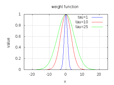
Further an additional parameter, controls the width of the weighting function. Higher the value of
, wider the weight function.

Figure: Plot of the exponential weighting function for different values of
Matlab/Octave code snippet
clear ;
close all;
x = [1:50].';
y = [4554 3014 2171 1891 1593 1532 1416 1326 1297 1266 ...
	1248 1052 951 936 918 797 743 665 662 652 ...
	629 609 596 590 582 547 486 471 462 435 ...
	424 403 400 386 386 384 384 383 370 365 ...
	360 358 354 347 320 319 318 311 307 290 ].';

m = length(y); % store the number of training examples
x = [ ones(m,1) x]; % Add a column of ones to x
n = size(x,2); % number of features
theta_vec = inv(x'*x)*x'*y;
tau = [1 10 25 ];
y_est = zeros(length(tau),length(x));
for kk = 1:length(tau)
	for ii = 1:length(x);
		w_ii = exp(-(x(ii,2) - x(:,2)).^2./(2*tau(kk)^2));
		W = diag(w_ii);
		theta_vec = inv(x'*W*x)*x'*W*y;
		y_est(kk, ii) = x(ii,:)*theta_vec;
	end
end

figure;
plot(x(:,2),y,'ks-'); hold on
plot(x(:,2),y_est(1,:),'bp-');
plot(x(:,2),y_est(2,:),'rx-');
plot(x(:,2),y_est(3,:),'go-');
legend('measured', 'predicted, tau=1', 'predicted, tau=10','predicted, tau=25');
grid on;
xlabel('Page index, x');
ylabel('Page views, y');
title('Measured and predicted page views with weighted least squares');

Observations
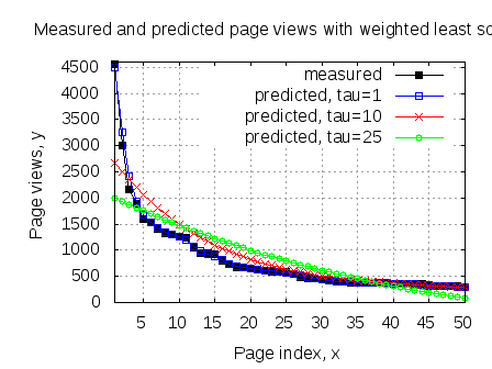
a) For a smaller value of (=1), the measured and predicted values are almost on top of each other
b) For a higher value of (=25), the predicted value is close to the curve obtained from the no weighting case.
c) When predicting using the locally weighted least squares case, we need to have the training set handy to compute the weighting function. In contrast, for the unweighted case one could have ignored the training set once parameter vector is computed.
References
CS229 Lecture notes1, Chapter 3 Locally weighted linear regression, Prof. Andrew Ng

