Phase noise power spectral density to Jitter

Following a brief discussion with my friend Mr. Rethnakaran Pulikkoonattu on phase noise profiles, he pointed me to his write up on Oscillator Phase Noise and Sampling Clock Jitter . In this post, we will discuss the math behind integrating the phase noise power spectral density (in dBc/Hz) to find the root mean square jitter value.

Jitter

In the post on ADC SNR with clock jitter we discussed about the effect of having incorrect sampling clock on the signal to quantization noise ratio. The error in sampling clock is caused by the variations on the timing of the signal. Jitter causes the the zero crossing of the clock to vary slightly from the desired location.

Figure : Clock with jitter

The clock with jitter can be expressed as,

,

where

 is the jitter in time

 is the equivalent phase jitter expressed in radians and

is the frequency of the clock.

The mean square value of phase jitter is computed as,

,

where

is the ratio of noise power in 1Hz bandwidth (BW) at offset from carrier to carrier signal power (recall from the post on oscillator phase noise)

The root mean square (rms) value  of the jitter is expressed as,

in radians and

in seconds.

Computing jitter from phase noise profile

The mean square value of jitter can be found by integrating the phase noise profile  over the frequency range. The phase noise profile  is typically specified in decibels, “decibels below carrier per hertz or dBc/Hz at a frequency   away from the carrier frequency “.

Phase noise profile

From the post on Oscillator phase noise, we know that

 (or equivalently -20dB per decade).

However due to other noise sources there are regions in the phase noise spectrum where  and so on, followed by a region where the phase noise power spectrum does not change with frequency. Typical phase noise profile follows a piece wise linear curve (with varying values of slope) between two frequency points as shown below.

Figure : Power spectral density of oscillator phase noise spectrum

The rms phase jitter can be computed from the phase noise profile as,

.

Area in the region A12

With the piece-wise linear assumption, the line connecting the regions  can be expressed as,

 ,

where

 is the slope and

 the constant.

.

The area is found by integrating over the frequencies from , i.e.

.

Note : 

Knowing that , the term

a)  and

b) .

The integration simplifies to,

.

When , using L’Hopital’s Rule and the knowledge that ,

.

Summarizing the area under the region A12 is,

.

Using the above approach, the area under each region can be found to compute the integrated power.

Example

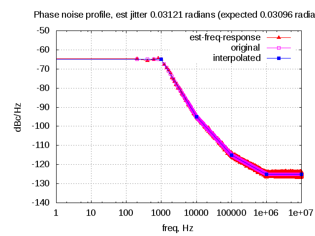
Consider a carrier of frequency 10MHz having an example phase noise profile having power spectral density (dBc/Hz vs frequency as follows).

Figure : Example phase noise profile

Click here to download Matlab/Octave script for computing the root mean square jitter (in radians and seconds) from the phase noise power spectral density profile.

For this example, can be seen that the integrated root mean square (rms)  jitter in radians is 0.018052 and corresponding to 287.32 pico seconds for a clock of 10MHz.

References

a) Pulikkoonattu, R. (June 12, 2007), Oscillator Phase Noise and Sampling Clock Jitter, Tech Note, Bangalore, India: ST Microelectronics, retrieved March 29, 2012

b) Phase Noise (dBc/Hz) to Phase Jitter (ps RMS) Calculator from JitterTime.com

c) List of Integrals from wikipedia

d) L’Hopital’s Rule in wikipedia

e) Derivative – entry in wikipedia